
There is a quiet crisis playing out inside every production AI system running today. It is not about model quality. The models are remarkably capable. The crisis is about memory — specifically, how much of it gets consumed the moment a model starts actually doing its job.
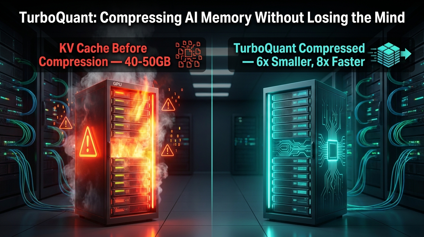
When a large language model generates a response, it does not recompute everything from scratch for each new token. It stores intermediate calculations — called keys and values — in a structure known as the KV cache, and it reads from that cache at every step of generation. The bigger the model, the longer the context window, the larger the batch of simultaneous users: the KV cache grows with all of it. For a 70-billion-parameter model handling an 8,000-token context at a batch size of 32, that cache can consume between 40 and 50 gigabytes of GPU memory before a single weight is even considered.
That is not a theoretical edge case. That is the everyday reality of serving a capable AI system to real users at scale.
Google Research’s answer to this problem — presented at ICLR 2026 — is a compression algorithm called TurboQuant. It compresses the KV cache to approximately 3.5 bits per value, achieving a 6x reduction in memory usage with statistically zero accuracy loss across a comprehensive battery of long-context benchmarks. On NVIDIA H100 GPUs, it delivers up to an 8x speedup in attention computation compared to a full 32-bit baseline.
This post goes deep on what TurboQuant actually does, how it achieves results that prior methods could not, what the benchmarks genuinely show, where it fits in the broader compression ecosystem, and what it means in practice for teams deploying AI systems at scale.
The Memory Wall: Why the KV Cache Breaks Everything at Scale
To understand why TurboQuant matters, you first need to understand the specific problem it solves — and it is a problem that sits at the intersection of architecture, hardware, and economics.
What the KV Cache Actually Is
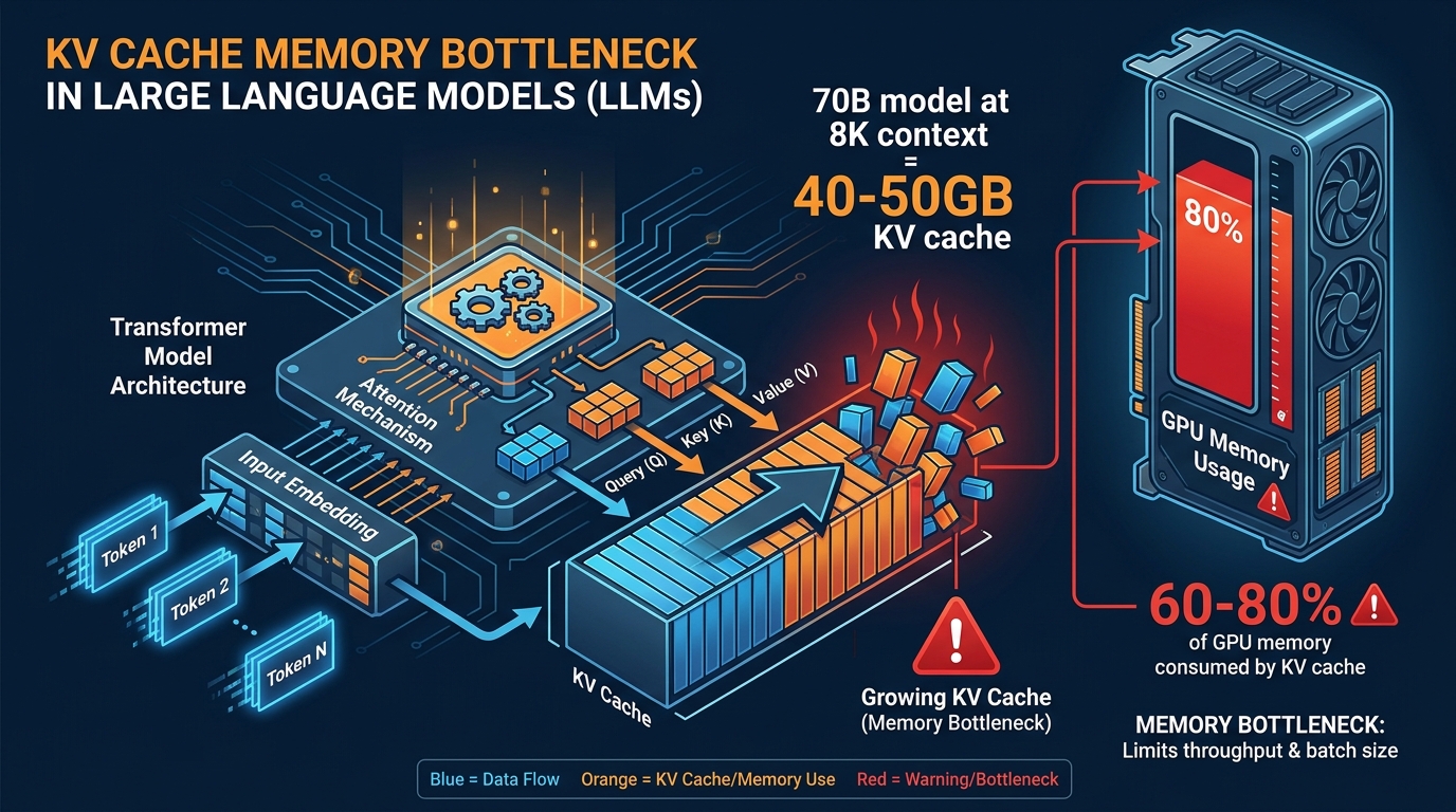
Transformer-based language models process text by computing attention over all previous tokens in a sequence. Each layer in the transformer maintains its own set of key (K) and value (V) vectors for every token it has processed. Rather than recomputing these from scratch with every new token generated, the model stores them in memory and retrieves them on demand. This is the KV cache.
In theory, it is an elegant optimization. In practice, it creates a memory footprint that scales with four simultaneous variables: sequence length, batch size, number of transformer layers, and the dimensionality of each attention head. None of these are small numbers in modern production systems.
How Bad the Numbers Actually Get
The math is unforgiving. A 70-billion-parameter model running at FP16 precision, with a 128-layer architecture and 8,000-token context window, serving a batch of 32 simultaneous requests, can require between 40 and 50 gigabytes of KV cache memory. That is the cache alone — not the model weights themselves, which add another 140 gigabytes in FP16.
Researchers estimate that the KV cache consumes between 60% and 80% of available GPU memory in typical long-context inference scenarios. This creates a cascading set of practical problems:
- Throughput collapses: Without memory optimization, serving throughput can drop 2x to 4x compared to theoretically possible rates, because memory constraints force smaller batch sizes.
- Context windows get truncated: Teams needing to serve 128K-token contexts discover they simply cannot without either massive multi-GPU infrastructure or painful quality tradeoffs.
- Infrastructure costs multiply: Adding context length or batch size often means doubling the number of GPU nodes — a direct multiplication of the inference bill.
- Latency spikes from I/O: When the KV cache exceeds available GPU VRAM, systems offload to CPU or disk, introducing latency spikes that make real-time applications unreliable.
Why This Problem Was Hard to Solve
The fundamental challenge with KV cache compression is that the keys and values are runtime data — they are computed dynamically from the input, not fixed parameters like model weights. You cannot calibrate a compressor on them beforehand, because you do not know what they will contain until the model is actually running. This rules out most standard post-training quantization approaches, which rely on calibration datasets to tune their codebooks.
Prior compression attempts either required knowing the data distribution in advance, introduced biases that degraded model accuracy on long-context tasks, or achieved compression at the cost of computational overhead that erased the speed gains. TurboQuant was specifically designed to solve this class of problem.
What TurboQuant Is and Where It Came From
TurboQuant is a vector quantization algorithm developed by Google Research and presented as a poster at the International Conference on Learning Representations (ICLR) 2026 on April 25, 2026. It was publicly introduced on March 24, 2026.
The algorithm targets one thing specifically: the KV cache. It does not touch model weights. It does not require retraining, fine-tuning, or any calibration data. It is entirely data-oblivious, meaning it makes no assumptions about what the vectors it is compressing will contain. It operates entirely on the mathematical structure of high-dimensional vectors — a property that turns out to be predictable enough to exploit very effectively.
The Theoretical Foundation
TurboQuant is built on two bodies of mathematical work that predated it but had not been combined in this way for KV cache compression: optimal scalar quantization theory and the Johnson-Lindenstrauss transform.
The key insight that makes TurboQuant possible is that when you take a high-dimensional vector from the unit hypersphere — which is exactly what normalized attention keys and values are — and rotate it randomly, something mathematically useful happens. The individual coordinates of the rotated vector converge toward a known Beta distribution (which approximates a Gaussian at higher dimensions). Because this distribution is known and fixed, you can build a precomputed optimal quantizer for it without ever seeing the actual data.
This means the compression codebook can be computed once, offline, and applied to any KV cache at inference time — no calibration, no data access, no model-specific tuning required.
Inside the Algorithm: How PolarQuant and QJL Work Together
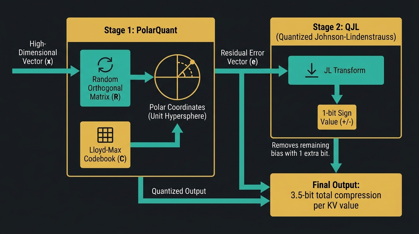
TurboQuant operates through a two-stage compression pipeline. Each stage addresses a distinct problem in the quantization process, and together they achieve compression quality that neither could reach independently.
Stage One: PolarQuant
The first stage is called PolarQuant. It handles the majority of the compression work and can be understood conceptually as converting a location description from Cartesian coordinates to polar coordinates.
In standard Cartesian space, describing a point requires specifying its distance along each independent axis. The values can vary widely, making them hard to quantize efficiently without knowing their range in advance. PolarQuant converts vectors on the unit hypersphere to polar coordinates instead — representing them by an angle and a magnitude, analogous to saying “go 5 blocks at a 37-degree angle” instead of “go 3 blocks East and 4 blocks North.”
Technically, this works by applying a random orthogonal rotation matrix to the input vector. This rotation — implementable efficiently via the Walsh-Hadamard transform at O(d log d) complexity — transforms the vector’s coordinate distribution into the known Beta distribution. A precomputed Lloyd-Max scalar quantizer, optimal for exactly that distribution, is then applied independently to each coordinate.
Because the quantizer is precomputed for a fixed, known distribution and requires no scaling based on the actual input values, there is no per-vector normalization overhead. The compression is both computationally light and mathematically near-optimal.
PolarQuant alone achieves strong compression — roughly 3 bits per KV coordinate — but it introduces a small systematic bias in the compressed representation. This bias is small enough to be acceptable in many settings, but it causes accuracy degradation in demanding long-context tasks, particularly those requiring precise retrieval over very long sequences. The second stage exists to fix this.
Stage Two: Quantized Johnson-Lindenstrauss (QJL)
The second stage, QJL (Quantized Johnson-Lindenstrauss), adds just one additional bit per value to the compressed representation — but that bit eliminates the residual bias introduced by PolarQuant almost entirely.
The Johnson-Lindenstrauss lemma is a classical result in mathematics proving that high-dimensional vectors can be projected into much lower-dimensional spaces while approximately preserving their pairwise distances. QJL applies this principle to the residual error between the original vector and its PolarQuant approximation. It projects that residual through a JL transform and stores only the sign bit (0 or 1) of the result.
That single additional bit provides an unbiased correction to the inner product estimates that the attention mechanism computes. The attention mechanism ultimately needs accurate inner products between query vectors and key vectors to compute attention scores — QJL ensures that the compression error does not systematically push those scores in any particular direction.
The combined effect of 3 bits from PolarQuant plus 1 bit from QJL gives TurboQuant its characteristic 3.5 bits per KV value compression target, with distortion within approximately 2.7 times the information-theoretic lower bound — a remarkably tight result for a training-free method.
Why “Data-Oblivious” Matters More Than It Sounds
The phrase “data-oblivious” may sound like a constraint, but it is actually TurboQuant’s greatest practical strength. Because the algorithm makes no assumptions about the specific model or input distribution, it can be applied immediately to any transformer-based model — Llama, Gemma, Mistral, or any architecture that follows the standard attention pattern — without any preparation step whatsoever.
There is no calibration run needed. No representative dataset to collect. No fine-tuning stage. No model-specific configuration to tune. A team can drop TurboQuant into an existing inference pipeline and have it working correctly on the first inference call. For production systems where fast iteration matters, this is a significant operational advantage.
The Benchmark Numbers: What the Research Actually Shows
The claims made for TurboQuant are specific enough to be falsifiable, and the evaluation methodology is broad enough to be meaningful. Here is what the research actually demonstrates.
Long-Context Benchmarks
Google evaluated TurboQuant across five major long-context evaluation frameworks, using Llama-3.1-8B-Instruct, Gemma, and Mistral-7B as test models.
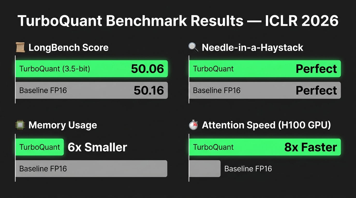
LongBench is a multi-task benchmark covering question answering, code completion, summarization, few-shot learning, and synthetic tasks over long documents. Llama-3.1-8B-Instruct with 3.5-bit TurboQuant scores 50.06 versus 50.16 for the uncompressed FP16 baseline — a difference of 0.10 points, well within normal benchmark variance. This is effectively indistinguishable performance.
Needle In A Haystack tests a model’s ability to retrieve a specific piece of information embedded within a very long document — the most demanding test of KV cache integrity, because a single compressed key or value that loses important information can cause a retrieval failure. TurboQuant achieves perfect scores on this benchmark, matching the uncompressed baseline exactly.
ZeroSCROLLS evaluates comprehension over very long documents where the model must integrate information from across the full context. TurboQuant results are statistically indistinguishable from uncompressed baselines.
RULER is a recently developed synthetic benchmark designed specifically to test long-range retrieval, multi-hop reasoning, and aggregation tasks over long contexts — tasks designed to stress-test exactly the kinds of errors that KV cache compression would introduce. TurboQuant passes all task categories without measurable degradation.
L-Eval covers long-document understanding including document QA, summarization, and reading comprehension. Again: statistically equivalent to the full-precision baseline.
Memory and Speed Numbers
The performance efficiency gains are more straightforward to measure:
- 6x+ KV cache memory reduction at 3–3.5 bits per coordinate, compared to FP16 at 16 bits per coordinate.
- 8x speedup in attention logit computation on NVIDIA H100 GPUs when comparing 4-bit TurboQuant to a 32-bit baseline. For FP16 comparisons, speedups range from 4x to 6x depending on context length and batch size.
- 128K-token context at 74GB for a 104-billion-parameter model — a context length and model size combination that would be prohibitively expensive or impossible without compression of this magnitude.
A Note on What “Zero Accuracy Loss” Means in Practice
Claiming “zero accuracy loss” deserves scrutiny. TurboQuant’s results are more precisely described as statistically indistinguishable from full-precision baselines across the evaluated benchmarks. The 0.10-point difference on LongBench is a real number — it is just smaller than the noise floor of the benchmark itself.
This matters because prior compression methods, including KIVI and the component algorithms PolarQuant and QJL operating independently, do show measurable accuracy drops at equivalent compression levels. TurboQuant’s combination of the two is specifically engineered to stay below the benchmark noise floor, not to claim an impossible perfection. That is a meaningful distinction.
TurboQuant vs. GPTQ, AWQ, and Weight Quantization: What’s Actually Different
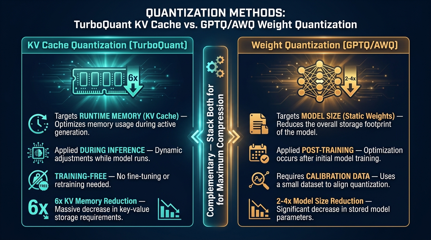
A persistent source of confusion in discussions of TurboQuant is the question of how it relates to the broader ecosystem of quantization methods — GPTQ, AWQ, SLiM, NVFP4, and others. The short answer is that TurboQuant targets a fundamentally different bottleneck, and the two classes of methods are complementary rather than competing.
Weight Quantization: What GPTQ and AWQ Do
GPTQ (Generalized Post-Training Quantization) uses Hessian-based calibration to reduce model weight precision, typically from FP16 to 4-bit integers. It requires a calibration dataset, takes time to apply, and reduces the static size of the model on disk and in GPU memory. A 70B model in FP16 consumes roughly 140GB; GPTQ at 4-bit brings this down to approximately 35GB.
AWQ (Activation-Aware Weight Quantization) takes a different approach — it identifies the roughly 1% of weights that are most sensitive to precision loss (by analyzing activation magnitudes) and protects those weights while aggressively quantizing the rest. AWQ consistently outperforms GPTQ on quality benchmarks at equivalent bit widths, achieving around 95% quality retention at 4-bit versus roughly 90-93% for GPTQ, while also delivering slightly higher throughput on optimized kernels.
Both methods target model weights — the static parameters that define what a model knows. They reduce the model’s memory footprint at rest, and at inference time they enable smaller VRAM requirements and higher throughput through faster weight-loading and denser compute.
What TurboQuant Targets Instead
TurboQuant targets the KV cache — the dynamic, runtime memory that grows with every token in the context. This is a categorically different bottleneck. A 7-billion-parameter model running at 4-bit weight quantization might need only 4-5GB for its weights, but at a 64K context length, the uncompressed KV cache can still consume 20-30GB.
Weight quantization does not help with this at all. The KV cache grows regardless of how aggressively the weights are compressed. TurboQuant addresses the half of the memory problem that GPTQ and AWQ leave untouched.
Stacking Both for Maximum Effect
The practical implication is that production deployments can — and should — use both approaches simultaneously. Apply GPTQ or AWQ to reduce the static model footprint, then apply TurboQuant to compress the runtime KV cache. The two compression mechanisms operate on entirely separate memory regions and do not interfere with each other.
A deployment combining 4-bit AWQ weight quantization with 3.5-bit TurboQuant KV cache compression can, in theory, run a 70-billion-parameter model with a long context window on infrastructure that would previously have required a model half that size. That represents a genuine shift in what is deployable on a given hardware budget.
Where TurboQuant Outperforms KIVI
The most direct prior comparison for TurboQuant is KIVI, an earlier KV cache quantization method. KIVI also targets the KV cache and applies low-bit quantization to reduce its size. In head-to-head comparisons on the benchmarks listed above, TurboQuant consistently outperforms KIVI — particularly on tasks requiring long-range retrieval and multi-hop reasoning, where KIVI’s quantization errors accumulate over long sequences in ways that TurboQuant’s bias-corrected approach avoids.
Real-World Deployment: What the Cost Savings Actually Look Like
Benchmark results from research papers are a starting point, not an endpoint. The more meaningful question for anyone operating AI systems is what TurboQuant-class compression actually does to the economics of production deployment.
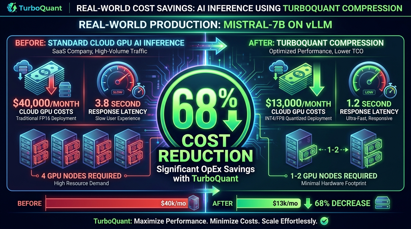
The SaaS Inference Cost Example
One of the more concrete production examples documented in early 2026 involves a B2B SaaS platform running an AI writing assistant built on a fine-tuned Mistral-7B model. The team was originally running the model via cloud GPU instances, spending approximately $40,000 per month on inference compute. Response latency averaged 3.8 seconds.
After compressing the model to 4-bit precision and self-hosting with vLLM, the monthly inference cost dropped to $13,000 — a reduction of 68%. Response latency fell to 1.2 seconds. The compression technique applied was consistent with TurboQuant-class KV cache quantization combined with weight quantization. The team retained the same hosted model with no degradation in downstream quality metrics.
This is not an isolated data point. Research across production deployments consistently shows 50-80% cost reductions per query from comprehensive compression strategies, with TurboQuant’s KV cache component accounting for a significant portion of that gain — particularly for workloads with long average context lengths.
The GPU Consolidation Calculation
Beyond per-query cost, memory compression changes the fundamental infrastructure equation. A deployment that previously required four H100 80GB nodes to handle a given throughput level — because the KV cache consumed most of available VRAM — may only require two nodes after TurboQuant compression, assuming the compression releases sufficient memory for larger batch sizes.
At current cloud GPU pricing, moving from four H100 nodes to two reduces compute costs from approximately $19.20 per hour to $9.60 per hour. Over a month of continuous serving (720 hours), that difference is nearly $7,000 — just from infrastructure consolidation, independent of any per-query savings from reduced memory bandwidth demands.
Context Window Economics
Perhaps the most underappreciated economic implication of TurboQuant is what it enables for context window pricing. Many AI API providers currently charge significantly more for requests using longer context windows, partly because longer contexts impose disproportionately larger memory burdens on their infrastructure.
With 6x KV cache compression, a 128K-token context has roughly the same memory footprint as a 21K-token uncompressed context. This changes the unit economics of long-context workloads fundamentally — making document processing, code review over large repositories, and extended conversation systems economically viable at scales that were marginal before.
Long-Context Inference: Why This Is Where TurboQuant Matters Most
If TurboQuant has a single most important application, it is enabling long-context inference at scale. The connection between KV cache compression and long-context capability is direct and mathematical: longer contexts produce larger KV caches, and larger KV caches are exactly what TurboQuant compresses.
What Changes at 128K Tokens
Modern capable models increasingly support context windows of 128,000 tokens or more. At this scale, the ability to process and reason over entire books, complete codebases, multi-hour transcripts, or large document sets becomes possible in a single model call. This is qualitatively different from the 4,000–8,000-token context windows that dominated AI applications just two years ago.
But supporting 128K contexts in production is not just a model capability question — it is an infrastructure question. Without compression, the memory requirements become prohibitive for all but the most well-resourced deployments. A 104B-parameter model handling a 128K-token context requires approximately 74GB for the KV cache alone at compressed (TurboQuant) rates. Without compression, the same cache would require over 400GB.
RAG and Document Processing Applications
Retrieval-Augmented Generation (RAG) systems that retrieve and inject large amounts of context into model inputs are perhaps the most direct industrial beneficiary of KV cache compression. Every additional retrieved document adds tokens to the context, which adds memory to the KV cache. With TurboQuant compression, teams can inject substantially more context per query before hitting memory limits — potentially improving answer quality by increasing the amount of relevant information available to the model at inference time.
The Needle In A Haystack benchmark results are directly relevant here: TurboQuant’s perfect retrieval scores on this test confirm that precise recall over long, compressed contexts is preserved. A system that compresses KV caches but introduces retrieval errors would be worse than useless for RAG applications. TurboQuant passes this test definitively.
Agentic Workflows and Extended Conversations
Agentic AI systems — those that operate over many steps, maintain conversation history, use tools repeatedly, and build up substantial context over long sessions — are among the most memory-intensive use cases in modern AI deployments. An agent running a complex research task might accumulate tens of thousands of tokens of context over the course of a single session. Without KV cache compression, every such session balloons in memory consumption.
TurboQuant makes sustained long-session agents economically viable without requiring per-session memory pruning strategies that force the model to forget earlier context. The ability to keep more context alive in compressed form without sacrificing retrieval accuracy has direct implications for the quality of agentic outputs.
Edge AI and On-Device Deployment: The Smaller-Model Angle
While TurboQuant’s highest-profile application is in large-scale inference on H100 clusters, it also has significant implications for the other end of the spectrum: deploying capable AI models on devices with limited memory.
The Edge Deployment Constraint
On-device AI — running models on smartphones, laptops, IoT devices, or embedded systems — operates under tight memory budgets that make model size the primary constraint. A device with 8GB of RAM cannot run a model that requires 16GB even after aggressive weight quantization, unless the runtime memory overhead can also be controlled.
The KV cache is part of that runtime overhead. On a phone handling a 4K-token conversation, an uncompressed KV cache for a capable 7B-parameter model might require 2-3GB of memory just for the cache. TurboQuant-class compression reduces this by 6x, bringing it under 500MB — potentially making the difference between a model that fits and one that does not.
Specific Small-Model Implications
For models designed specifically for edge deployment — architectures in the 1B–7B parameter range that have become standard for on-device tasks — the KV cache can represent an even larger fraction of total runtime memory than it does for large server models. Weight quantization on small models is already well-developed (GGUF formats for consumer hardware are mature), but KV cache quantization for edge contexts is a more recent and active area.
TurboQuant’s training-free, data-oblivious approach is particularly attractive for edge deployment because the implementation complexity is low. There is no edge-specific calibration step needed, no model-specific tuning, no fine-tuning pipeline to maintain. The same algorithm that compresses KV caches for Llama-3.1-8B on an H100 cluster applies equally to a 3B-parameter model running on an NPU in a consumer device.
What TurboQuant Cannot Do: Honest Limitations
No compression method is universally beneficial, and responsible evaluation of TurboQuant requires acknowledging where it does not help and where its approach has genuine constraints.
It Does Not Reduce Model Weight Size
TurboQuant compresses the KV cache — not the model parameters. For use cases where the primary constraint is model download size, storage footprint, or the VRAM consumed by model weights (rather than KV cache), TurboQuant does nothing. A team trying to reduce the size of a model for distribution to end users still needs GPTQ, AWQ, GGUF, or another weight quantization approach.
Short-Context Workloads See Limited Gains
For workloads with very short context windows — a few hundred tokens per request — the KV cache is not the dominant memory consumer, and compressing it by 6x does not fundamentally change the system’s memory profile. TurboQuant’s gains scale with context length; for short-context high-throughput scenarios (such as classification or very short-form generation), the primary bottleneck is elsewhere.
The Decoding Speed Profile
The 8x speedup figure in TurboQuant’s benchmarks refers to attention logit computation specifically — the inner product calculations between queries and compressed keys. This is a meaningful portion of overall inference time for long-context scenarios, but it is not the whole picture. Prefill throughput (how fast the model processes the initial prompt) shows different speedup profiles than decode throughput (how fast it generates tokens one by one). Teams benchmarking end-to-end latency in production should measure carefully rather than applying the 8x figure universally.
Hardware-Specific Implementation Quality
The benchmark speedup numbers were measured on NVIDIA H100 GPUs using optimized CUDA kernels. On different hardware — AMD GPUs, older NVIDIA architectures, custom AI accelerators — the speedup profile will differ and depends heavily on the quality of the low-level implementation. The compression ratio and accuracy properties are hardware-independent, but the speed gains require hardware-tuned kernels to fully realize.
The Broader Compression Landscape: Where TurboQuant Sits in 2026
TurboQuant does not exist in isolation. It is part of an active and rapidly developing field of AI model efficiency research, and placing it in context helps clarify both its significance and its limitations.
The Multi-Dimensional Compression Stack
Modern AI efficiency work in 2026 operates across multiple dimensions simultaneously:
- Weight quantization (GPTQ, AWQ, SLiM, NVFP4): Reduces model parameter precision. Well-matured for 4-8 bit targets. NVFP4 represents NVIDIA’s hardware-native format for H100/H200 accelerators, with software-hardware co-design for maximum throughput.
- KV cache quantization (TurboQuant, KIVI, FP8 KV): Reduces runtime attention memory. TurboQuant currently leads on quality-vs-compression tradeoff at 3-4 bit targets.
- KV cache eviction (StreamingLLM, H2O, SnapKV): Rather than compressing the cache, these methods selectively discard KV entries that are statistically less likely to influence future attention. Orthogonal to quantization — can be combined with TurboQuant for extreme memory reduction.
- Speculative decoding: Uses a smaller draft model to propose multiple tokens that a larger model verifies in parallel. Targets latency rather than memory. Compatible with all compression approaches.
- Architectural efficiency (MQA, GQA, MLA): Multi-Query Attention, Grouped-Query Attention, and Multi-head Latent Attention reduce the number of KV heads in the first place, reducing the cache at the source. TurboQuant compresses whatever cache these architectures produce.
The Convergence Toward 3-4 Bit Targets
A notable trend across 2026’s efficiency research is the convergence toward 3-4 bit quantization as the practical sweet spot for both weight and KV cache quantization. Below 3 bits, accuracy degradation becomes difficult to compensate for with residual correction techniques at current algorithmic maturity. Above 4 bits, memory savings become insufficient to justify the engineering overhead. TurboQuant’s 3.5-bit target sits precisely at this emerging consensus sweet spot.
The Road Toward 2-Bit and Below
Research into sub-3-bit quantization is active, with methods like QuIP# and AQLM pushing weight quantization toward 2-bit targets with acceptable accuracy on selected benchmarks. Whether similar approaches can work for KV cache quantization — where the data-oblivious constraint adds difficulty — is an open research question. TurboQuant’s theoretic distortion bound of 2.7x the information-theoretic minimum suggests there may be room for improvement, but the required techniques may need to move beyond training-free approaches.
What Engineering Teams Should Take From TurboQuant
For practitioners working on AI systems rather than AI research, the technical details above translate to a set of concrete operational considerations.
When TurboQuant Should Be Your First Optimization
If your system’s primary constraint is GPU memory — not model quality, not weight size, but the VRAM available for running inference — and if your workloads involve long context windows (8K tokens or more), TurboQuant-class KV cache compression should be near the top of your optimization list. The training-free, zero-calibration deployment model means time-to-value is very low.
Profile your inference runs to confirm that KV cache memory is actually the binding constraint before investing in the implementation. For short-context high-volume workloads, other optimizations (batching strategy, weight quantization, serving framework tuning) may yield better returns.
The Combination Play
The maximum benefit comes from combining TurboQuant with weight quantization rather than treating them as alternatives. A practical deployment stack for a mid-sized language model in 2026 looks roughly like: AWQ or GPTQ at 4-bit for model weights + TurboQuant at 3.5-bit for KV cache + PagedAttention via vLLM for memory allocation efficiency. These three layers operate on different parts of the memory hierarchy and compound without significant interaction effects.
Benchmark Your Specific Workloads
TurboQuant’s accuracy results are compelling across standard long-context benchmarks, but production AI systems have their own specific accuracy requirements. Before deploying KV cache compression in a system where accuracy degradation has direct consequences — medical, legal, financial applications — run TurboQuant against your actual workload distribution and accuracy thresholds. The algorithm’s data-oblivious design means you cannot guarantee benchmark performance will transfer perfectly to every input distribution — only testing can confirm acceptable behavior.
Watch the Hardware-Specific Implementation
The speedup gains from TurboQuant require optimized kernel implementations for your specific hardware. If you are running on H100s with well-maintained inference software (vLLM, TensorRT-LLM, or similar), the kernels may already be available or in development. On less common hardware configurations, you may get the memory savings without the full speed gains until community implementations catch up.
Conclusion: The Economics of AI Are Being Rewritten in Bits
TurboQuant is not a product announcement. It is a research result — a carefully validated demonstration that it is possible to compress the runtime memory footprint of large language model inference by 6x, with no accuracy loss on demanding benchmarks, using a completely training-free algorithm that can be applied to any transformer-based model in production today.
The reason this matters is not primarily technical. The reason it matters is economic. The KV cache is one of the primary reasons that deploying capable AI systems at scale costs what it costs. It is why inference currently consumes 55-80% of enterprise GPU spending. It is why extending context windows from 8K to 128K has historically meant multiplying infrastructure budgets by a factor of 10 or more. It is why teams that want to serve AI to millions of users still need to make painful choices between model capability, context length, batch size, and infrastructure spend.
TurboQuant does not eliminate those tradeoffs. But it moves the constraint significantly. The same GPU budget that previously supported a given deployment configuration can now support a configuration with 6x more effective context capacity. The same context window that previously required six GPU nodes may now require one.
Combined with mature weight quantization methods, efficient serving frameworks, and architectural improvements like grouped-query attention that have already halved baseline KV cache sizes in newer model families, TurboQuant is one piece of a broader efficiency stack that is steadily making the per-token cost of AI inference fall — not by making the models less capable, but by compressing the computational overhead without compressing the intelligence.
For any team running language models in production, that is worth understanding in detail — because the details determine which problems you can actually afford to solve.
Key Takeaways
- TurboQuant compresses the KV cache to 3.5 bits per value — a 6x reduction from FP16 — with zero measurable accuracy loss on five major long-context benchmarks.
- It operates training-free and data-obliviously via a two-stage process: PolarQuant (polar coordinate rotation + Lloyd-Max scalar quantization) followed by QJL (1-bit Johnson-Lindenstrauss residual correction).
- The 8x attention speedup on H100 GPUs is real but specific to attention logit computation with optimized kernels — end-to-end latency improvements vary by workload.
- TurboQuant is complementary to, not competing with, weight quantization methods like GPTQ and AWQ. Stack both for maximum memory efficiency.
- The biggest practical beneficiaries are long-context workloads: RAG systems, document processing, extended agentic sessions, and 128K+ token context deployments.
- Real-world deployments report 50-80% inference cost reductions when comprehensive compression stacks are applied. KV cache compression is a meaningful contributor to that range.
- For short-context workloads, other optimizations will likely yield greater returns first.