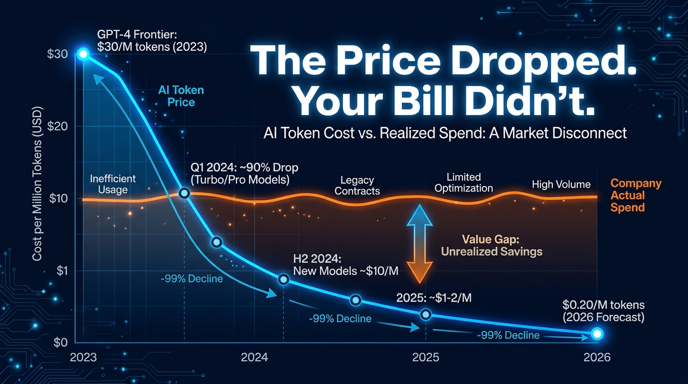
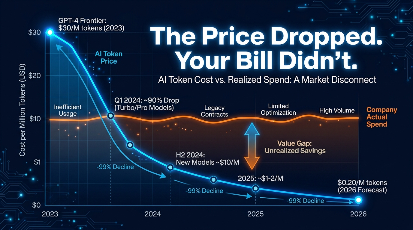
Token prices have collapsed. OpenAI cut its GPT-5.6 Luna model by 80% — from $1.00 to $0.20 per million input tokens — in a single announcement. DeepSeek followed with a 75% permanent reduction on its V4-Pro API. Google’s Gemini 2.5 Flash sits at $0.075 per million input tokens, a fraction of what frontier model access cost eighteen months ago. By any measure, inference has never been cheaper.
And yet, most engineering teams haven’t seen their AI bills move much.
That gap — between the market’s dramatic price compression and your organization’s actual spend — is not a pricing problem. It is an architecture problem. The economics of AI inference have changed faster than the systems built to consume it. Teams are still routing every request through a single premium model, still stuffing entire document corpora into context windows, still re-processing identical system prompts on every call. The model got cheaper. The code didn’t.
This guide is for the engineers, platform architects, and technical leads who want to close that gap. Not with surface-level prompt tips, but with the layered architectural changes that compound on each other to deliver 80% or greater cost reduction — while maintaining, or in some cases improving, the quality of outputs your users depend on.
We’ll work through five distinct optimization layers, show how they stack, and look at the governance model that keeps them from degrading over time.
The 2026 Pricing Landscape: What Actually Changed and Why It Matters
To understand why architectural redesign matters more than ever, it helps to understand what’s driving the price compression — because the underlying forces determine which optimizations will hold and which will be superseded.
The Price War in Numbers
The most significant recent moves are worth cataloguing clearly, because the scale of the drops is easy to underestimate:
- OpenAI GPT-5.6 Luna: Input tokens dropped from $1.00 to $0.20 per million (80% cut). Output tokens fell from $6.00 to $1.20 per million. This model sits in the mid-tier — capable enough for a wide range of production tasks, now priced at sub-budget-model rates from two years ago.
- OpenAI GPT-5.6 Terra: Input tokens dropped 20% to $2.00 per million. Output tokens fell to $12.00 per million. Terra represents the first meaningful price movement on OpenAI’s upper-mid tier.
- OpenAI Sol (frontier): The flagship model received a 20%+ reduction, a sign that price competition is now affecting even the models organizations treat as untouchable.
- DeepSeek V4-Pro: A 75% permanent cut on API access, pushing input tokens to approximately $0.0035 per million for cached tokens — making it among the lowest-cost capable models available via API today.
- Gemini 2.5 Flash: Sitting at roughly $0.075 per million input tokens and $0.30 per million output tokens, Flash is the baseline against which many teams now benchmark their model spend.
- GPT-4o mini / GPT-4.1 mini: Still anchored at $0.15 per million input tokens and $0.60 per million output tokens, with cached input at $0.075 per million — representing strong value for repetitive, structured workloads.
What’s Driving the Drops
These price cuts are not charity. They reflect genuine efficiency improvements: advances in speculative decoding, hardware utilization at massive scale, and increasingly efficient quantization techniques that allow models to run at lower precision without meaningful capability loss. The cost to serve a token has fallen materially, and competitive pressure among providers is forcing those savings to be passed through to customers.
The important implication: this compression is likely to continue. Which means a system architected to take advantage of today’s pricing will be progressively more valuable as the floor drops further. The investment in architectural optimization pays dividends not just now, but at every future price level.
The Hidden Problem with Cheaper Models
Cheaper models create a specific temptation: simply swap your current model for a cheaper one and declare victory. Some teams have done exactly this — and discovered that the quality-to-cost tradeoff didn’t hold the way they expected. Cheaper models are cheaper for a reason. Routing everything indiscriminately to the lowest-cost option is how you introduce quality regressions that are hard to detect until they’ve already damaged user trust.
The right approach is selective — and that selectivity requires architecture, not just a configuration change.
Why Most Teams Are Still Leaving 70% of Savings on the Table
Before diving into the optimization layers, it’s worth diagnosing why the gap between available savings and realized savings is so large. The patterns are remarkably consistent across organizations.
The Single-Model Monolith
The most common anti-pattern: a single model handles every request in a product. The model is typically chosen for the hardest use case — complex reasoning, nuanced tone, multi-step analysis — and then applied uniformly to tasks that don’t need anywhere near that capability. A user asking a simple factual question gets the same model as one asking for a multi-document synthesis. The organization pays frontier rates for routine work.
In practice, across most production LLM workloads, 60-70% of requests are classifiable as “simple” or “templated” — factual lookups, structured extractions, standard summaries, route-able support queries. These do not need a frontier model. They need a reliable, fast, cheap model. Most systems don’t make that distinction.
Context Amnesia
Every token sent into a model costs money. Context that is sent but not needed is money burned. In agentic and conversational systems, context accumulates with every turn — and most implementations send the full conversation history on every call, even when 80% of that history is irrelevant to answering the current question.
The same problem appears with retrieval: many RAG implementations over-retrieve, stuffing far more document context than the model needs to answer the query accurately. More context is not always better. It is always more expensive.
Cache Blindness
Prompt caching — the ability to reuse the computed key-value states of repeated prompt prefixes — is now a first-class feature supported by OpenAI, Anthropic, and Google. It can reduce the cost of cached tokens by up to 90%. And yet most systems are not structured to take advantage of it, because they haven’t structured their prompts so that the stable parts come first and the variable parts come last. A small architectural decision at prompt design time translates into massive ongoing savings.
Output Verbosity as a Cost Driver
Output tokens are consistently more expensive than input tokens — often by 3x to 5x across providers. A model that writes a 1,200-word response when a 200-word response would serve the use case equally well is consuming 6x the output token budget for no functional benefit. Most systems don’t constrain output length explicitly, don’t use structured output schemas to eliminate wrapper prose, and don’t distinguish between contexts where verbosity adds value and contexts where it doesn’t.
Layer 1 — Model Tiering and Intelligent Routing
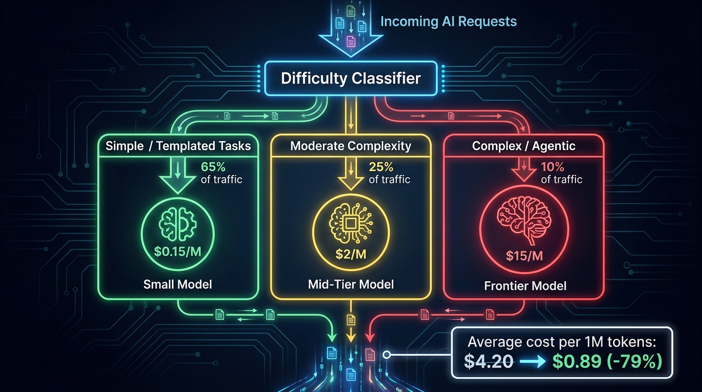
Model routing is the highest-impact single lever available to most engineering teams. Production deployments that implement proper multi-tier routing consistently report 30-85% cost reductions, with the strongest results pushing toward the upper end of that range on workloads where a large proportion of requests are classifiable.
How Tiered Routing Works
The core principle is simple: match the capability requirement of the task to the cost profile of the model that can handle it adequately. Build three tiers:
- Tier 1 — Lightweight models ($0.075–$0.20/M input tokens): Gemini 2.5 Flash, GPT-4o mini, GPT-4.1 mini, DeepSeek V4-Pro cached. Suitable for classification, extraction, templated responses, simple Q&A, content moderation, intent detection.
- Tier 2 — Mid-tier models ($0.80–$2.00/M input tokens): Claude Haiku 4.5, GPT-5.6 Luna at new pricing, GPT-4.1. Suitable for moderate-complexity tasks — summarization of medium-length documents, structured analysis, multi-step reasoning on bounded problems.
- Tier 3 — Frontier models ($3.00–$15.00/M input tokens): Claude Sonnet/Opus, GPT-5.6 Terra/Sol, Gemini 2.5 Pro. Reserved for tasks that genuinely require high-capability reasoning — complex multi-document synthesis, novel problem-solving, high-stakes output generation where quality is non-negotiable.
The Classifier Layer
Routing requires a classifier — something that evaluates an incoming request and assigns it to a tier before dispatching it. There are several viable approaches:
Rule-based routing is the simplest: define request categories in your application logic, and route each category to a designated model tier. A customer support flow might route “order status” queries to Tier 1, “returns policy disputes” to Tier 2, and “legal/compliance escalations” to Tier 3. This requires no ML but demands well-structured application logic and breaks down when requests are free-form.
LLM-as-classifier uses a small, cheap model (typically Tier 1) to evaluate each request and assign a difficulty score or category. The classifier prompt is short and its output is a simple label. The overhead of the classification call is typically recovered within the first few routed calls. Research from LMSYS-style routing benchmarks (RouteLLM) showed up to 85% cost reduction while maintaining approximately 95% of GPT-4-level quality on MT-Bench.
Embedding-based routing uses semantic similarity to match requests to predefined query clusters, each mapped to a model tier. This can be faster than LLM classification and handles nuanced categorization well, but requires upfront cluster definition and embedding infrastructure.
Real-World Routing Results
A documented example from the customer support domain: a platform routing factual and templated tickets to Claude Haiku while escalating complex disputes to Sonnet saw monthly spend drop from approximately $42,000 to $18,000 — a 57% reduction with no measurable change in ticket resolution quality. The routing logic added roughly two weeks of engineering time. The payback period was under a month.
More aggressive routing setups — combining provider-side routing with application-level classification and caching — report 80-95% cost reductions on highly structured workloads where a large fraction of requests are templated or low-complexity. The key variable is what proportion of your traffic is genuinely simple: if it’s 60% or more, routing alone can get you close to the 80% target without touching anything else.
Guard Rails for Routing Quality
Routing introduces quality risk if the classifier over-routes complex requests to simpler models. Protect against this with output quality monitoring: track downstream signals like user re-queries, escalation rates, and human override rates. Set threshold rules that escalate to a higher tier when a lower-tier model’s output fails a confidence or format check. Build in a “re-route on failure” path from day one.
Layer 2 — Prompt Caching: The 90% Savings Nobody Is Using
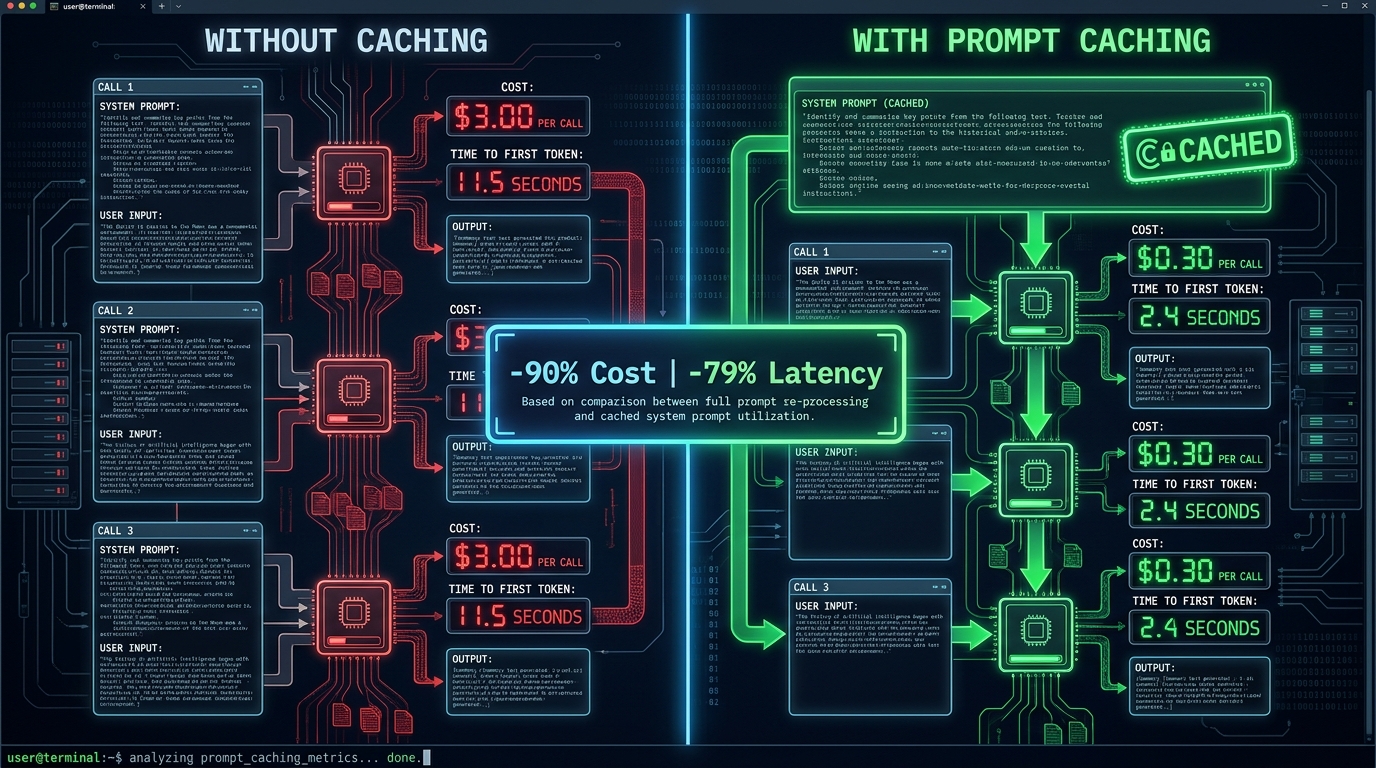
Prompt caching is the most consistently underutilized cost lever in production LLM systems. The savings are real, provider-supported, and activated by an architectural decision — not a new technology purchase. Yet the majority of teams deploying LLMs at scale have not structured their prompts to benefit from it.
How Prompt Caching Works
When a model processes input tokens, it computes intermediate key-value (KV) states — the mathematical representations the model uses to understand relationships between tokens. Normally, these states are discarded after each call. Prompt caching preserves those states for repeated prompt prefixes, so subsequent requests sharing that prefix pay only for the new, variable portion of their input.
The economics are striking:
- Anthropic (Claude): Cached reads cost 10% of the base input token price. Cache writes cost 25% more than the base rate. If you cache a prefix and reuse it twice, you’ve already broken even. By the tenth reuse, you’ve saved 78.5% versus processing without caching.
- OpenAI: Prompt caching is enabled by default for supported models. Cache reads cost 10% of the standard uncached input rate. For GPT-5.6 and later, cache writes cost 1.25× the standard rate. A prefix written once and reused nine times costs 2.15× total versus 10× without caching.
- Google (Gemini): Context caching is available for Gemini 1.5 Pro and Flash, with cached tokens billed at a fraction of standard input rates.
Anthropic’s published benchmarks for Claude show: a chat-with-a-100,000-token-book workflow achieving 90% cost reduction and 79% latency reduction. Many-shot prompting with a 10,000-token prompt shows 86% cost savings and 31% latency improvement. Multi-turn conversations show 53% cost reduction.
Structuring Prompts for Cache Hits
The critical architectural principle: stable content must come before variable content in your prompt. Cache breakpoints work from the beginning of the prompt outward. If variable user content appears before your static system instructions, the cache can never match — because the prefix changes on every call.
The correct structure follows this order:
- System instructions (persona, rules, constraints, output format specifications)
- Tool definitions and schemas (function calling definitions, JSON schemas)
- Static context (background documents, knowledge base content, few-shot examples)
- Conversation history (prior turns, which grows over time)
- Current user input (always last, always variable)
Any change in the prefix before a cache breakpoint invalidates the cache for everything after it. This means your system prompt should be frozen and not dynamically constructed on each call. Even small differences — a whitespace character, a variable instruction — break the cache hit.
Semantic Caching: Handling Similar (Not Identical) Queries
Provider-level prompt caching handles exact prefix matches. Semantic caching goes further — it identifies requests that are semantically similar to previous ones and returns a cached response rather than making a model call at all.
Semantic caching typically sits in front of your LLM API and uses embedding similarity to find near-matches in a cache store. When a new query’s embedding falls within a defined similarity threshold of a cached query, the cached response is returned directly. The savings can be substantial for high-repetition workloads — support bots, FAQ systems, product description generators — where many users ask functionally identical questions in slightly different words.
The trade-off is precision: semantic caching introduces the risk of returning an approximate answer to a subtly different question. Cache hit thresholds need to be calibrated carefully, and certain query types (factual, time-sensitive, personalized) are poor candidates for semantic caching regardless of similarity scores.
Layer 3 — Context Window Discipline
Context window management has emerged as one of the primary cost levers in 2026 — and it’s one of the least visible, because the waste accumulates gradually rather than appearing as a discrete line item. Large context windows are a capability you pay for whether or not you use them effectively. The cost scales linearly with tokens sent: sending 10x the context costs 10x more, regardless of whether any of that additional context affected the output.
The RAG vs. Full-Context Decision
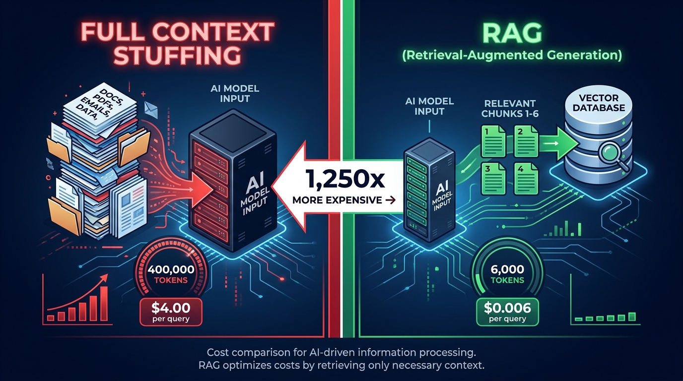
The most consequential context decision for teams building over large knowledge bases is whether to use retrieval-augmented generation or full-context stuffing. The cost difference is not marginal — it can be orders of magnitude.
Published estimates for 2026 workloads are stark: a 400,000-token full-context prompt costs approximately $4.00 per query on a mid-tier model, uncached. A RAG implementation retrieving the six most relevant chunks — approximately 6,000 tokens — costs approximately $0.006 per query. That is a 1,250× cost difference for a single query type.
This does not mean RAG is always the right choice. Full-context approaches have genuine advantages for small, stable knowledge bases where the entire corpus fits in a modest context window, for synthesis tasks where relationships across the full document set matter, and for one-off analysis where retrieval infrastructure overhead isn’t justified. But for high-volume, dynamic knowledge bases queried repeatedly, RAG is not an optimization — it’s a necessity.
Conversation History Trimming
In conversational applications, context bloat is insidious. Every turn adds tokens. By turn 20 of a conversation, the system may be sending 15,000 tokens of history to answer a question that requires only the last two turns as context. The oldest turns are often irrelevant, and the model’s attention mechanisms may be paying little effective attention to them anyway.
Practical history management strategies include:
- Sliding window: Keep only the last N turns in context. Simple to implement, trades recency for history depth. Works well for single-session conversational UIs.
- Summarization compression: Periodically summarize older conversation segments into a compact summary, replacing the raw turns with the summary. Preserves key context at a fraction of the token cost.
- Hierarchical memory: Separate “working memory” (recent turns, active task context) from “long-term memory” (key facts established earlier in the conversation, stored in a retrieval system and fetched on demand). Only inject long-term memory when the current query’s semantics suggest it’s needed.
- Selective history: Track which past turns were actually referenced in model outputs, and deprioritize turns that have never been referenced during context trimming.
Retrieval Quality as a Cost Lever
In RAG systems, retrieval quality directly determines cost efficiency. Poor retrieval — fetching too many chunks, fetching loosely relevant chunks, failing to filter by recency or authority — inflates the context sent to the model without improving output quality. Investing in better retrieval (improved embedding models, hybrid search combining dense and sparse retrieval, re-ranking layers that filter before context injection) reduces the token burden on the LLM and improves the signal-to-noise ratio of what it receives.
A useful heuristic: if your retrieval returns chunks that the model ignores, your retrieval is too broad and you’re paying for noise. Tighten chunk size, improve re-ranking, and measure retrieval precision not just recall.
Long-Context Economics: When to Flip the Equation
There is a scenario where full-context loading wins on cost: when your knowledge base is small and stable, and you run many queries against it within a session. With prompt caching enabled, loading a 50,000-token document corpus once and caching it can make subsequent queries extremely cheap — just the user’s question and the model’s response, with the document corpus served from cache at 10% of standard token rates. In this scenario, full-context plus caching beats RAG on both cost and latency. Know your query pattern before choosing your architecture.
Layer 4 — Output Control and Structured Generation
Input tokens get most of the attention in cost conversations, but output tokens are typically 3x to 5x more expensive per token across major providers. A team spending $10,000 per month on inference where 40% of that cost is output tokens has a $4,000 line item that can be substantially reduced through output discipline.
The Verbosity Problem
Left unconstrained, LLMs tend toward verbosity. They add caveats, restate the question, provide context the user didn’t ask for, structure responses with headers that weren’t requested, and pad toward perceived completeness. This is not a model defect — it reflects training on human content that often rewards thoroughness. But for production applications, verbosity is a cost driver and often a UX problem simultaneously.
The fix is explicit instruction. In your system prompt, specify the desired response length, format, and level of detail. Not as guidance — as a constraint. “Respond in 2-3 sentences only” is more effective than “keep responses concise.” Setting the max_tokens parameter as a hard cap prevents runaway outputs on edge cases. Evaluating a sample of production outputs for verbosity patterns and targeting the highest-verbosity prompt categories for explicit constraints is straightforward to do and consistently delivers cost reductions.
Structured Outputs vs. Free-Form JSON
When your application needs machine-readable output, the choice between structured outputs (schema-enforced generation) and JSON mode (valid JSON, no schema enforcement) has both cost and reliability implications.
Structured outputs — where the model is constrained to generate output matching an exact schema — tend to produce shorter responses because they eliminate the prose wrapper that often surrounds JSON in JSON mode responses (“Here is the requested JSON:”). They also eliminate retry loops caused by schema violations, which consume additional tokens and latency. The operational cost savings — fewer retries, less parsing failure handling, no downstream correction loops — often exceed the direct token savings.
The design principle is to make your schemas as minimal as possible. Every optional field in your schema is an invitation to the model to generate content. Define only the fields your application actually consumes. Avoid deeply nested structures where flat structures would serve as well. Test your schemas against production traffic patterns and trim aggressively.
Reasoning Token Budgeting
Models with visible reasoning steps (chain-of-thought, extended thinking modes) generate reasoning tokens that are billed before the final answer. For complex problems, these reasoning tokens are often what makes the difference between a correct and incorrect answer. For simple problems, they are pure cost overhead.
OpenAI’s GPT-5 family supports a “minimal reasoning effort” mode that produces very few or no reasoning tokens, keeping output token counts tightly correlated with response verbosity. Using high-reasoning modes on tasks that don’t require deep reasoning is one of the more expensive anti-patterns in current LLM deployments. Map your task categories to appropriate reasoning effort levels and enforce those mappings in your routing logic.
Layer 5 — Batching, Async, and Off-Peak Scheduling
Not every LLM request needs to return a response within two seconds. A significant portion of production AI workloads are asynchronous by nature — report generation, content enrichment pipelines, bulk classification, nightly summarization jobs, data transformation workflows. For these use cases, there is no user waiting on the other end of the call. Yet many teams run them through the same synchronous, low-latency API path as interactive features — and pay premium prices for a latency guarantee they don’t need.
Batch APIs and Their Discounts
OpenAI’s Batch API offers a straightforward deal: accept up to 24-hour processing latency and pay 50% of the standard API price. For asynchronous workloads, this is a direct cost halving with no architectural complexity beyond queuing your requests and polling for results. Anthropic offers similar message batching through its API. These discounts are real and consistent — they don’t require negotiation or volume commitments.
The organizational friction is usually process, not technology: getting product teams to accept that a bulk classification job or content enrichment pipeline can run overnight rather than in real time. Once that expectation is set, the technical implementation is typically a few hours of work.
Request Aggregation and Throughput Optimization
For synchronous workloads, batching individual tokens into larger requests can improve throughput efficiency and reduce per-request overhead. Many providers optimize their infrastructure for batched inference — larger batches amortize fixed serving costs across more tokens, and providers pass some of this efficiency back in throughput-optimized pricing tiers.
At the application layer, request aggregation means collecting short-lived requests that arrive in close temporal proximity and processing them together rather than individually. This is most effective for high-volume, low-latency-tolerance pipelines — recommendation scoring, content moderation queues, classification pipelines — where individual requests are small and predictable.
Speculative Decoding and Inference Runtime Efficiency
For teams running self-hosted or dedicated inference infrastructure, speculative decoding represents a meaningful throughput improvement. Speculative decoding uses a small “draft” model to propose multiple future tokens, which the larger “target” model then verifies in parallel — effectively reducing the number of serial decoding steps required. Published benchmarks show 2x to 4x throughput improvements on many workloads, translating directly to lower cost-per-token for self-hosted inference.
At the API level, you don’t control speculative decoding directly — providers implement it internally. But understanding that some providers use it more aggressively than others helps explain why the cheapest-per-token model is not always the cheapest-per-task, once latency and throughput constraints enter the equation.
Stacking the Layers: What 80% Actually Looks Like in Practice
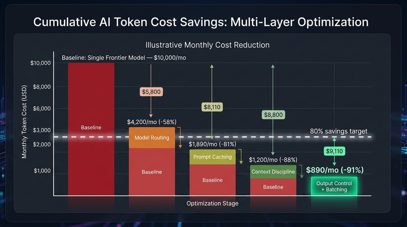
The five layers described above don’t operate independently — they compound. The order of implementation matters because some layers unlock savings in others, and the combined effect is non-linear. Here’s how a realistic stacking scenario plays out for a hypothetical mid-size production deployment.
The Baseline
Starting point: a product team running all LLM calls through a single frontier model (priced at ~$10/M input, $30/M output). Monthly spend: $10,000. Traffic is a mix of simple classification tasks, moderate summarization, and occasional complex analysis. System prompt is 3,000 tokens, reconstructed dynamically on every call. Conversation history is sent in full. Output length is unconstrained.
After Layer 1: Model Routing
Traffic analysis reveals: 62% of requests are simple classification or templated response tasks, 28% are moderate-complexity, 10% are genuinely complex. Implement a classifier and route accordingly — Tier 1 for 62%, Tier 2 for 28%, frontier for 10%.
Result: average input cost per million tokens drops from ~$10 to ~$2.30. Average output cost drops proportionally. Monthly spend: approximately $4,200 (-58%).
After Layer 2: Prompt Caching
Restructure prompts so the 3,000-token system prompt is a stable prefix on every call. Enable caching at the provider level. Cached reads cost 10% of input rates. With an average of 15+ requests per session, cache hit rates average ~85%.
Result: effective input token cost drops by ~76% on cached portions. Monthly spend: approximately $1,890 (-81% from baseline).
After Layer 3: Context Window Discipline
Implement conversation summarization after turn 8, replacing earlier history with a 200-token summary. Replace bulk context stuffing with RAG, reducing average context injection from 12,000 tokens to 2,800 tokens per call.
Result: average tokens per request drops by ~35% on top of the already-reduced baseline. Monthly spend: approximately $1,200 (-88% from baseline).
After Layer 4: Output Control
Add explicit length constraints to system prompts for each routing tier. Implement structured outputs for all machine-readable endpoints. Eliminate verbose reasoning modes from Tier 1 and Tier 2 tasks.
Result: average output token count per request drops by ~40% on Tier 1 tasks, ~25% on Tier 2. Monthly spend: approximately $950 (-90.5% from baseline).
After Layer 5: Batching Overnight Async Work
Move nightly enrichment pipeline (roughly 15% of monthly volume) to batch API at 50% discount. Monthly spend: approximately $890 (-91.1% from baseline).
The 80% target is comfortably exceeded before reaching the final layer. The incremental gains from each layer vary by workload — routing delivers the most for high-volume mixed-complexity traffic, caching delivers most when system prompts are large and stable, context discipline delivers most when conversations are long or knowledge bases are large. The key is accurate assessment of where your specific costs are concentrated before deciding which layers to prioritize.
AI FinOps: Governance, Attribution, and Token Budgets
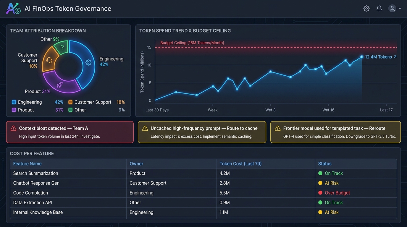
Architectural optimization is not a one-time event. Token costs erode over time as teams add features, prompts grow, new models get adopted inconsistently, and successful product features scale in ways that weren’t anticipated. Without a governance layer, your initial 80% savings will be partially recaptured by entropy within six to twelve months.
Token Attribution by Feature and Team
The foundation of AI FinOps is attribution. Every LLM call in production should be tagged with metadata that identifies the product feature, the team responsible, the model used, and the routing tier. This data, aggregated in a cost monitoring dashboard, makes cost anomalies visible before they become budget problems.
Without attribution, cost optimization is guesswork. With it, you can answer: which feature is responsible for 40% of frontier model spend? Which team’s recent deployment doubled context window usage? Which caching optimization is underperforming on hit rate? Attribution is the difference between reactive cost firefighting and proactive cost management.
Token Budgets and Policy Enforcement
Once attribution exists, budgets become actionable. Define per-feature token budgets — both soft limits (alerting) and hard limits (throttling or automatic tier downgrade when exceeded). These budgets serve multiple purposes: they force product teams to think about LLM cost at design time, not after deployment; they prevent single features from unilaterally consuming disproportionate inference budget; and they create visibility into cost-per-feature that product managers can use to assess whether a feature’s cost is justified by its value.
Policy enforcement can be implemented at the API gateway level: a middleware layer that checks token budgets before dispatching calls, enforces routing rules, applies caching logic, and logs metadata. This centralizes cost governance rather than distributing it across individual feature implementations — where it tends to be applied inconsistently or ignored under delivery pressure.
Continuous Prompt Auditing
Prompts drift. System prompts accumulate instructions added for edge cases that no longer occur. Tool definitions grow as APIs evolve. Few-shot examples multiply without pruning. A quarterly prompt audit — reviewing every production system prompt for redundant instructions, outdated context, and token waste — consistently finds optimization opportunities that have accumulated since the last review.
Automate the detection layer: log prompt lengths and flag any system prompt that exceeds a defined token ceiling for human review. Track cache hit rates by endpoint — a falling hit rate on a previously stable endpoint is a signal that something in the prompt has changed and broken the cache prefix.
The LLM Cost Review Cadence
Treat LLM cost review as a regular operational discipline, not a one-off project. Monthly: review token spend by feature and team, investigate anomalies, check cache hit rates. Quarterly: audit system prompts, review routing classifier performance, evaluate whether the model tier pricing has shifted enough to warrant reassignment. Annually: reassess the full architecture against the current pricing landscape — what was optimal at current prices may need adjustment as prices continue to compress.
What Not to Cut: Preserving Quality Where It Matters
A cost optimization guide that doesn’t address quality risk is incomplete. The 80% savings target is achievable without meaningful quality degradation — but only if you’re deliberate about where the cuts happen.
Tasks That Require Frontier Models
Some task categories genuinely require the capabilities that only frontier models currently provide. These include:
- Complex reasoning chains where the problem space is novel and multi-step, and errors cascade through subsequent reasoning. Mathematical derivations, legal analysis, complex debugging across large codebases.
- High-stakes outputs where quality errors have material consequences — medical information synthesis, compliance documentation, contract review. The cost of a frontier model call is trivial compared to the cost of acting on a flawed output.
- Novel creative generation where the quality difference between tiers is perceptible and consequential to the product experience — flagship content generation, nuanced tone-matching in brand contexts.
- Low-volume, high-sensitivity agentic tasks where an agent will take real-world actions based on the output and mistakes are expensive to reverse.
The routing tier logic should be configured conservatively for these categories — if in doubt, escalate to a higher tier. The cost of over-routing complex tasks to frontier models is measured in cents. The cost of under-routing them is measured in user trust and potential downstream errors.
Monitoring Quality, Not Just Cost
Every cost optimization should have a paired quality signal. When you implement routing, measure response quality before and after by sampling outputs across tiers and running evaluations. When you tighten output length constraints, check that downstream tasks depending on those outputs still receive adequate information. When you reduce context, verify that task accuracy metrics haven’t degraded.
The goal is a Pareto-optimal operating point — maximum cost savings at or above the quality floor required for the use case. If an optimization reduces quality below that floor, the savings are illusory: you’ll spend them back in user churn, support escalations, or the engineering time needed to fix the output quality problem.
Evals as Infrastructure
The teams that sustain cost optimization over time without quality degradation share one characteristic: they have evaluation infrastructure in place before they optimize. An eval suite — automated tests measuring task accuracy, format compliance, and output quality across representative inputs — makes it safe to change routing rules, swap models, or tighten prompts, because you can verify the impact immediately rather than discovering it from user complaints.
Building evals is engineering work, and it’s tempting to skip when the optimization opportunity looks obvious. Resist that temptation. The architectural changes that deliver 80% cost savings also carry architectural risk. Evals are the safety net.
The Architecture Is the Price Negotiation
The framing most organizations bring to AI cost management is transactional: negotiate better rates, find a cheaper provider, wait for prices to drop. Those strategies have merit at the margins. But the data is clear that the difference between an organization capturing 80% of available savings and one capturing 10% is not the vendor contract — it’s the architecture.
The five layers described in this guide — model tiering and routing, prompt caching, context window discipline, output control, and batching — are each individually capable of delivering meaningful savings. Stacked together, with the right sequencing and governance, they consistently reach the 80% threshold that has become the benchmark for mature AI cost management in 2026.
What makes this moment particularly significant is the rate of change in the underlying pricing landscape. OpenAI’s 80% cut on Luna, DeepSeek’s 75% reduction, the continued compression of Gemini Flash pricing — these are not anomalies. They reflect genuine efficiency improvements in model serving that will continue. Teams with well-architected systems will benefit from every future price drop automatically. Teams relying on a single model at flat rates will continue to pay above market for what they could be getting for less.
Practical Starting Points
If you’re approaching this architecture for the first time, prioritize in this order:
- Audit your traffic. Pull 30 days of LLM call logs. Classify request complexity. If more than 50% of your traffic is simple or templated, routing is your highest-ROI first move.
- Restructure your system prompts. Move all static content to the top. Enable provider-level prompt caching. This takes hours and pays back in days.
- Measure context per request. Find your 95th percentile context size. That number tells you how much waste exists in your current context management approach.
- Add output constraints to your highest-volume endpoints. Even a 30% reduction in average output length on your top five endpoints will be visible in your monthly spend.
- Identify your async workloads. Any pipeline that runs on a schedule, rather than in response to a live user request, is a candidate for batch API pricing.
None of these steps require purchasing new tooling, negotiating new contracts, or waiting for the next model release. They require engineering time and a clear-eyed assessment of where your current architecture is wasting money. The price war is in your favor. The question is whether your architecture is positioned to capture what’s already on offer.